Folding Towels, Measured in Yen per Hour
We put advantage-conditioned learning (RECAP) on a real dual-arm robot and cut towel-folding cycle time by 4 seconds (over 5%); success rate barely moved. Every result is measured in profit per robot-hour.

Head of ML Engineering
Contents
This is the first post in a technical series about the ML work we do at Omotenashi Robotics. Future posts will each cover one experiment; this one starts with who we are and how we think, then walks through a full experimental arc we recently completed with advantage-conditioned policy learning (RECAP [1]) on a real dual-arm robot.
66.7%
Success rate needed to break even
61%
Where we are. 6–10 points to go
4s+
Cycle time cut by RECAP
1. What we are building
We are not building a robot that can do everything. We are building robots that do one industry's work well enough to be deployed, as fast as possible.
The industry we chose is linen supply — the businesses that wash, fold, and deliver the towels and sheets used by hotels and hospitals. The work is physically repetitive, labor is chronically short, and the tasks are concrete enough to measure. Our robots fold more than face towels — bath towels, bath mats, wiping towels, gowns — and the roadmap extends beyond folding to other steps of the linen workflow. This post focuses on one task among them: folding face towels, picked one at a time from a pile, folded twice, and stacked.
Betting on a specific industry changes how you do ML. A general-purpose robot is judged by breadth of ability; ours is judged by whether a linen factory makes money running it. That single criterion drives everything below.
2. Goals in yen per hour
"Success rate 90%" is not a business goal by itself. We reduce every research goal to one number: the profit one robot generates per hour,
P = u · Z − c_itv · I
where Z is throughput (towels finished per hour), I is intervention frequency (times per hour a human must step in), u is the labor cost saved per towel a robot folds (for face towels we assume ¥10), and c_itv is the cost of one intervention (we assume ¥30). A finished towel saves the labor it would have taken; an intervention consumes labor somewhere else in the factory.
Throughput and intervention frequency follow from the two quantities we actually measure in evaluation: success rate p and cycle time. With a 120 s attempt limit and 60 s assumed per intervention, the expected time per towel is C = p · C_succ + (1 − p) · (120 + 60), where C_succ is the cycle time of a successful attempt, and then Z = 3600 / C, I = (1 − p) · Z. Note that Z is 3600 / C regardless of the success rate because we assume the human finishes the towel during the 60 s intervention — one towel per cycle, success or failure (that labor is what c_itv pays for).
The profit formula P = u · Z − c_itv · I is worth rewriting once. Substituting I = (1 − p) · Z into P gives
P = Z · (u − c_itv · (1 − p))
— and since Z > 0, the sign of P is decided by the success rate p alone. The break-even point is p* = 1 − u / c_itv = 1 − 10/30 = 66.7%. Until we cross it, success rate is the only variable that matters; cycle-time reduction only converts into profit once p exceeds 66.7% — in the red, spinning faster just spins the losses slightly faster too. For reference, a robot that folds nothing at all (p = 0%) exists only to call for an intervention every three minutes: P = −¥400/h. Read every number below against these two marks — −¥400/h and ¥0/h (p = 66.7%).
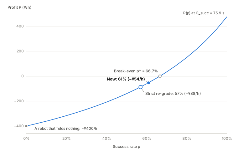
As you will see below, P is currently negative. But that red ink can also be read as the price we pay to collect real-robot data: whatever the success rate, an hour of operation yields the same amount of data — which is exactly why the −¥400/h of p = 0% makes the right comparison. It is the list price of that data collection, and the smaller the loss, the more cheaply we are collecting the same data. Today the robot is, in effect, an apprentice paying for its own training data. We publish these numbers internally for every experiment, because which improvement actually helps depends on the operating point — and can run against intuition. The formula forces that into the open; we will see a live example in §4.4.
3. How we do research
Every research activity exists to move P. When a new ML method is the bottleneck, we build one. But novelty itself is not the goal: improving how we collect data, fixing a camera mount, or applying a published method carefully often moves P more than inventing something. The RECAP story below is a case study in what "applying a published method carefully" actually means: controlled baselines, offline metrics designed before training, and honest accounting of what worked and what did not.
4. Case study: advantage-conditioned learning (RECAP) on towel folding
4.1 Why we care about RECAP
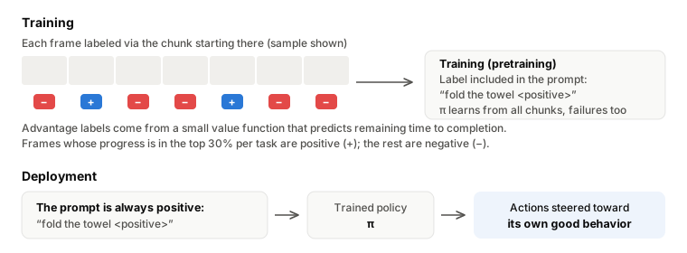
RECAP is the training recipe behind Physical Intelligence's π*0.6 [1]: label each training frame with a binary advantage indicator — did the next chunk of recorded behavior (a chunk being the short, contiguous sequence of actions a policy outputs in one inference call) make faster-than-usual progress ("positive") or not ("negative") — include that label in the policy's prompt during training, and at deployment always ask for "positive". The policy learns from all data, including failures, but is steered at inference toward its good behavior. Strictly speaking, RECAP in the paper names the full iterated loop: collect rollouts → update the value function → retrain the policy. What we tested in this post is its first turn; the iteration is still ahead of us (§6).
For us this maps directly onto P: better action selection should raise success rate (fewer interventions), and preferring fast-progress behavior should shorten cycle time (more throughput). That is why we consider it one of the most important methods in our pipeline, and why we tested it thoroughly rather than just running it once.
Our base policy is π0.5 [2] (openpi [4]), trained with real-time-chunking latency conditioning [3] throughout. This is why the motion in the videos above is smooth, with no visible stutter between action chunks: by simulating inference latency during training, the policy learns to commit to actions under the delays it will face at deployment. The advantage labels come from a small value function trained to predict normalized time-to-completion — the advantage of a frame is whether the predicted value 50 frames later rises more than the passage of time alone would explain, binarized at the top 30% per task. The paper itself switches to a cruder estimate during pretraining — the episode's realized return to the end against the predicted value — but we use this same 50-frame estimate consistently in both pretraining and finetuning.
4.2 Conditioning at finetune time only
We first ran the loop the cheap way: no conditioning in pretraining, value-function indicators injected only during task finetuning on demos plus the policy's own rollouts (episodes recorded by running the trained policy itself on the robot). Success rate did not improve. To separate "is the indicator derivation the problem?" from "is the policy training failing to use it?", we swapped the labels for human-annotated good/bad intervals on 100 rollouts and finetuned again — no better. Worse: even the unconditioned BC control (BC = behavior cloning, plain imitation learning with no conditioning) trained on the same demo+rollout mix landed well below a baseline trained on demos alone. In other words, mixing failure rollouts into imitation is costly all by itself, and the conditioning recovered none of it. Checking offline confirmed the picture: flipping the condition between positive and negative barely moved the generated actions — the conditioning was practically inactive.
The cause was the label's information content. A simple linear classifier taking the model's own observation embeddings as input predicts the label with AUC 0.92. A state that looks like it is about to fail almost always comes with recorded actions that do fail, so only a small fraction of frames carry label information independent of the observation — and that leaves no learning pressure to read the prompt. The fix: labels that carry information the observation does not already contain, learned where conditioning can take root — in pretraining.
4.3 The indicator moves into pretraining — offline checks before the robot
Following the π*0.6 recipe [1], we put advantage conditioning into pretraining. To be precise, our pretraining is a second pretraining: it starts from π0.5's public parameters and, in effect, finetunes them on our full pretraining set (3,000 episodes, over 100 tasks — see §5) — distinct from the pretraining Physical Intelligence ran to produce π0.5's original parameters. Running this for 20k steps with value-function indicators, the conditioning clearly activated: flipping the condition visibly moves the generated actions, and under "positive" the action chunks travel ~8% farther per chunk — the offline sign of shorter cycle times.
The remaining worry was that task finetuning would erase it. Finetuning on all-positive demo data — this is exactly the SFT stage of the π*0.6 recipe, where the paper fixes the indicator to positive — weakens the conditioning substantially, but mixing in 50 "recovery" episodes (the operator deliberately fails, then recovers — our own device: a cheaper way to collect failure-and-recovery behavior than live expert interventions) with real labels preserves it, with no side effect on imitation quality (it matches the BC control). Having confirmed the conditioning survives, we went to the robot.
4.4 On the robot
We evaluated on the robot in two stages. First came the configuration matching the paper's SFT stage — finetuned on all-positive demos only — against its BC control: success rate 56% vs 52%, successful cycle time 76.6 s vs 72.5 s (throughput 29.5 vs 29.0 /h, interventions 13.0 vs 13.9 /h, P = −¥95/h vs −¥127/h). Success rate edged up while cycle time actually lengthened — a small, ambiguous difference, consistent with the conditioning decay we had seen offline (this pair has not been re-graded under the unified criterion described below). The main event is the demo + recovery configuration whose conditioning we had confirmed intact:
| Success rate | Successful cycle time | Throughput Z | Interventions I | P = 10·Z − 30·I | |
|---|---|---|---|---|---|
| RECAP (as judged on site) | 61% | 75.9 s | 30.9 /h | 12.1 /h | −¥54/h |
| BC control (as judged on site) | 54% | 84.9 s | 28.0 /h | 12.9 /h | −¥107/h |
| RECAP (re-graded, single criterion — reference) | 57% | 72.1 s* | 30.4 /h | 13.1 /h | −¥88/h |
| BC control (re-graded, single criterion — reference) | 53% | 76.3 s* | 28.8 /h | 13.5 /h | −¥118/h |
* Cycle times in the re-graded rows are fold-completion times measured mechanically from the recordings. They exclude the delay between completion and the judge stopping the recording, so this yardstick reads shorter than the recording lengths in the as-judged rows.
Taken at face value: +7 points success, 9 s faster, a ¥53/robot-hour profit gap. We did not take it at face value. Each evaluation cell (method × robot) had been judged by a different person, and the judges' pass criteria turned out to differ widely — above all in how much corner offset and wrinkling they tolerated in a finished fold before counting it a success — a confound large enough to explain the entire success-rate gap.
So we had an AI re-grade all 200 demo + recovery episodes under one strict criterion: only tidy folds count as success. Concretely, we cropped the overhead-camera image from the final frame of each episode's recording, shuffled them with only a serial number so that method, robot, and judge could not be identified, assembled them into contact sheets, and gave them to the AI with the instruction: "Count as success only a completed state of two neat folds (almost no layer offset, wrinkles, or protruding corners); count everything else — folds with visible defects, or incomplete — as failure."
That is the "re-graded, single criterion" pair of rows in the table. The success-rate gap shrinks to 57% vs 53% (p-value 0.67) — no statistical difference. The cycle-time improvement, by contrast, survives every cut (at least 4 s even after removing judge-dependent components). Note that where exactly the pass line should sit is itself not yet settled — which is why these rows are reference values, and why fixing the criterion is the job of the AI-unified evaluation described in §6.
Honest summary: in the main demo + recovery configuration, RECAP shortened cycle time by at least 4 s (5%) and did not change success rate measurably. And held against the formula in §2, these two must not be weighted backwards. At the current operating point, one point of success rate moves P by about +¥9/h, while one second of cycle time works out to about ¥0.3/h in the wrong direction. Until we go profitable, success rate is the only variable that matters — and this reduction is a saving that starts paying dividends the moment p crosses the 66.7% break-even. We stand at 61% (57% under the strict re-grade) — 6 to 10 points from break-even. Measured from the −¥400/h of a robot that folds nothing, roughly 80% of the loss is already gone.
4.5 What this arc taught us
- What we banked: a robust cycle-time reduction of at least 4 s. But as §2's formula says, it converts into profit only past the 66.7% break-even. Success rate has not moved yet.
- Put the indicator in pretraining. Injected only at finetune time, it never worked.
- Keep negatives in the finetune mix, or the conditioning fades.
- The label is the battleground. Labels readable from the observation leave no learning pressure — that is why the conditioning of §4.2 stayed inactive.
5. The pretraining data, briefly
Everything above sits on an in-house pretraining set: about 3,000 teleoperated episodes across more than 100 tasks on our dual-arm platforms (two Nova5 arms each) — towels, pillowcases, and cloth in many configurations (spreading, folding, untwisting, recovering from bad states), plus a few non-linen manipulation tasks. Three cameras (overhead + both wrists). Training, pretraining and finetuning alike, runs on the NVIDIA RTX PRO 6000 Blackwell Workstation Edition. It is small by foundation-model standards and deliberately dense around the states our deployment tasks visit. How we collect and scale it — including simulation-generated data — is a topic for another post.
6. What's next
The current bottleneck is not subtle: about 20% of attempts time out, mostly in repeated grasp-misses where the gripper closes just short of the towel. Six to ten points of success rate separate us from the 66.7% break-even — §2's formula says to push there first. The fixes we are weighing include raising prediction accuracy on the method side, or effectively capturing and using depth information on the camera side — but we will isolate the cause before committing to one. In parallel, three things: AI-unified evaluation to kill judge variance for good (and to settle the re-grading criterion of §4.4), trying intervention data in the RECAP loop, and scaling pretraining — both more data and more training steps.
We are a small team; the person who runs this kind of experiment also designs the metrics, argues about the label definition, and stands next to the robot when it counts. If measuring robot learning in yen per hour — and publishing the negative results along with the positive — sounds like your kind of research culture, we are hiring ML engineers. We are looking for people who do not just use ML methods, but have the mathematical depth to genuinely understand the methods they work with — not to implement, report a number, and stop, but to analyze the results and choose the next move with precision. Come fold towels with us.
References
- [1]Physical Intelligence. π*0.6: a VLA That Learns From Experience. arXiv:2511.14759, 2025.
- [2]K. Black et al. (Physical Intelligence). π0.5: a Vision-Language-Action Model with Open-World Generalization. arXiv:2504.16054, 2025.
- [3]K. Black, A. Z. Ren, M. Equi, and S. Levine. Training-Time Action Conditioning for Efficient Real-Time Chunking. arXiv:2512.05964, 2025.
- [4]Physical Intelligence. openpi. GitHub, 2025.

We are hiring ML engineers
We judge research not by novelty, but only by whether it moved the goal that matters. If that sounds like your research culture, a conversation is enough to start. We also take enquiries about joint research and technical partnerships here.
Cite this article
BibTeX. Paste it straight into your reference manager.
@misc{omotenashi-recap-towel-folding-2026,
  author = {Kanta Sugiyama},
  title  = {Folding Towels, Measured in Yen per Hour},
  year   = {2026},
  url    = {https://omotenashi-robotics.com/en/research/recap-towel-folding},
  note   = {Omotenashi Robotics Research}
}